Shooting the Crab


Around midnight on Christmas Eve, I was texting with my brother and a friend in California when my phone started chiming. I was thrilled to see that Flickr had promoted my most recent astrophoto to their page! This is where they highlight 500 images selected from their daily haul of about one million. Even placed well “below the fold,” my photo would receive over 5,000 views by the New Year. About one viewer in 50 “faves” the image and each time this happens, an angel gets its wings…. Er, no, that doesn’t actually happen, but my phone vibrates, and I get a pleasing hit of dopamine, which added greatly to my holiday cheer!
While nerdy social media glory was not part of my original plan for astrophotography, posting in Flickr and Instagram costs me little but adds a couple of important dynamics to my hobby. First is some discipline – when I start processing my data it’s with the thought that I’m trying to reach an endpoint at which the image is good enough to share. Otherwise processing can sprawl indefinitely and my hard drive would continue to fill up with incomplete projects.
Second is having a handy catalogue of my images. By posting the “Tech Stuff” with each finished image, I’ve maintained a cloud- based catalogue dating back to mid-2014—within a few days of my retirement, not coincidentally—which is relevant to this shaggy crab story. Let’s go back in time to my early days of astrophotography to see if I’ve learned anything useful.
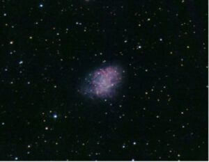
I like my first attempt at M1 (Fig. 2) for a few reasons.

Never mind that I had not yet figured out how to focus consistently. The first big item here is recognizing that this weird ghostly shape may not remind you of any crabs you’ve encountered, but to me it looks a LOT more like a crab than my recent shot looking like an Alien Easter Egg. With less color and definition of the nifty lacework of debris still holding together after nearly a thousand years, this version speaks to us regarding some of the fascinating history of this celestial object.
A thousand is not a round number I just pulled out of a hat. A hundred years ago, the nebula was definitively linked to a stellar explosion recorded as a supernova by Chinese and Japanese astronomers in 1054 CE. But the 18th and 19th century astronomers who characterized and named the nebula didn’t know that. Even though the nebula was first noted in 1731 by John Bevis, it first took on importance when Charles Messier’s encountered it about 30 years later. Frustrated that he was observing a fixed object rather than a more exciting comet, he was inspired to create his famous catalogue of faint fuzzies. The designation of Messier 1 or M1 arises from the coincidence that it just happened to be in the section of Taurus where Messier was searching for Halley’s Comet, and thus was first in his catalogue. I suspect that whatever Messier observed through his 4-inch scope from downtown Paris looked more like this 2014 image than anything else you’ll find in this article.
Incidentally, I’m confirming these factoids via , and I highly recommend the entry on the Crab Nebula. It includes a lot more information about its unusual and ever-changing astrophysics. Rather than rewrite the article here, I want to emphasize only how the Crab has evolved as an astrophotography target for me. But do check it out: there’s a lot going on up there.

My next imaging attempt about a year later (Fig. 3) came out much closer to my current take. I had learned a lot and changed much my gear and technique during those 12 months. By using a newer and improved CCD camera, a 0.5X focal reducer, a couple of light pollution filters, and the knowledge gained from a 5-day PixInsight workshop, I was now creating images which resembled those of typical backyard astrophotographers. Not the best, mind you but good enough to move up from a dismal zero to three!
The next image from two years later (Fig. 4) is not really any better. But this version used a different approach – a monochrome CMOS camera with red, green, and blue filters. The high focal length Questar still needed guiding, and processing the individual layers from individual filters was a small project. But the progress here relates to the much greater efficiency for capturing the data with a monochrome CMOS versus color CCD camera: Individual exposures were 12 seconds each versus 10 or 20 minutes; and total exposure time was dropped to 2.5 hours from six. Less than half the capture time and five faves!
Two more years passed while I converted most of my imaging to small refractors and very short exposures. My Questar is a Maksutov Cassegrain reflector, with impeccable optics in a very compact format. A few years in, my deep dive into the hobby taught me that no type of telescope is ideal for all purposes. The Questar’s native focal length of 1600 mm, even with the limited 3.5” aperture, is ideal for observation and imaging of solar system targets – especially the gas giants, Mars, the Sun and the Moon. But the combination of a high focal length and small aperture are very inefficient for deep sky imaging. The “focal ratio” of focal length divided by aperture is used for astro as well as terrestrial photography as a measure of the “speed” of an optical system, and Questar’s f/16 (1600-mm/90-mm) is something of a joke when it comes to deep sky. So I moved on to faster refractive optics – lenses which are nearly useless for Jupiter but great for faint fuzzies.

This next one (Fig. 5) was shot through my Borg 71FL at f/5.9. The Borg fits on a go-to mount that facilitates target acquisition and re-alignment. The SharpCap live-stacking technique lets me accumulate data from 4-second or 8-second exposures, which are so short there is no tracking error which would show in longer exposures as elongated stars. Conventional wisdom says to shoot the longest exposures your gear will allow under given sky conditions, because faint details will be lost in noise if your exposures are too short. But cooled CMOS cameras have a very low noise profile and consequently we can stack 100 6-second exposures in a way that is equivalent to one 600-second exposure. In this case I shot 4-second exposures, which were stacked and saved every four minutes. I then brought 23 stacks into PixInsight, processing them as though they were 4-minute exposures into one integrated image. Total exposure time 92 minutes. In Flickr I got nine Faves!
The 2019 image also used a color camera with a nebula filter. Around 2016 suppliers started making “dual band” filters which only pass the same wavelengths as individual narrowband filters for H-alpha (red associated with hydrogen alpha spectral line) and OIII (blue associated with doubly-ionized oxygen). These dual-band filters were specifically designed to facilitate narrowband-type imaging with color CMOS cameras, dramatically improving the efficiency of imaging from light-polluted locales. My IDAS LPS-V4 filter is a little more permissive and gives me fine results on nebular targets from the Bortle 7 red zone conditions of my Yonkers backyard.
With some powerful new features of PixInsight in the mix, I can say that this was my easiest Crab image. No guiding, easy target acquisition, no filter changes, one set of color images collected and processed in one night. And while my final image only had a minimal blue (oxygen) content, I was able to show off the complex internal filaments in red.
That 2019 image just preceded the pandemic; I’ve done plenty of imaging in the ensuing two years without returning to the Crab until just before Christmas 2021. We had a rare break in a long stream of overcast nights – but during a brilliant full Moon. I likened the moonlight to organic broccoli: it may be natural but it’s still broccoli. The full Moon may be a beautiful subject on its own but it still generates city level light pollution. So I decided to shoot with narrowband filters, and an H-alpha layer of M1 fit the bill. It came out well (Fig. 6)!

In this case I also wanted to take advantage of the latest improvements in SharpCap and PixInsight. Computer power is the other driver of change for backyard astrophotography.
SharpCap now includes some advanced mount control features. This means my $400 CubePro mount can be repositioned with a few clicks of a mouse. Compared with the complicated process I’d go through positioning my Questar on an invisible target in 2014, this feels like magic. The trick involves calling a plate-solving routine which compares an image to a full sky database and reveals with great accuracy where the telescope is pointed. When it’s working properly, I can re-center the scope on a target with literally one mouse click. It’s amazing and it makes imaging with backyard gear that much more efficient.
Notice that I managed to squeeze more lacy detail out of the 420-mm focal length Borg than the old 1600-mm Questar images. How? An important step was drizzle integration allowing me to “upscale” the resolution threefold. Drizzle is routinely used in planetary imaging to impute values between pixels when you stack frames with small variations in positioning on the sensor. The technique worked well with this dataset enabling me to zoom in and crop down to just a small portion of the frame without making the target look “pixelated” or “blocky.”
When the crystalline clear sky returned the next night, I shot two hours of OIII, which I combined with the Hα layer, resulting in the image at the beginning of this article (Fig. 1).
With 123 faves and counting, I’m going to need a good reason to shoot at M1 again in 2023! Maybe I’ll have a new camera or that robotic mount I’ve been coveting for a few years… we’ll see…