How far away is a Quasar? Using spectroscopy to find out
Distances in space are very difficult to measure accurately because of the extreme scales and limited practical resources available for space exploration. As a result, scientists have been forced to adapt different methods to try and gauge and measure the vast stellar distances across the universe. Measuring the distance to a nearby object like the Moon is easy and can be done with very high accuracy using radar. Yet, when we try to measure the distance to the nearest star, Alpha Centauri, if we used radar we would need to wait over 8 years for the radio waves to go there and come back, so instead astronomers use a geometry concept called parallax. Parallax is easy to visualize: stick your finger out and close one eye, then open the other eye, closing the first. The jumping in the location of your finger is due to the changed perspective of your left versus right eye. Extending this to astronomy, if we measure a nearby star in June and then again in December we can use the distance from the Earth to the Sun as one side in our triangle, and then calculate the distance to the star (Figure 1).
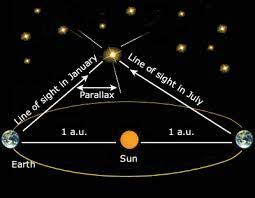
Figure 1. Measuring distance: Parallax
This works fine, until about 50 or so lightyears out, because at greater distances the base side of the Earth’s orbit is so little as to make the calculation very inaccurate. About 100 years ago astronomers discovered a few other methods to measure greater distances. They found certain types of variable stars or even supernova explosions that could help them measure out to 500 or so light years. But that is still not very much when you think about the scale of the universe being 15 billion light years or more!
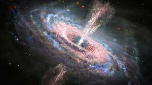
Quasars were discovered in 1960; today we know these objects as among the most energetic sources in the universe. A typical quasar is about 100 trillion times brighter than our sun! A quasar is basically a black hole that has an incredibly fast spinning cloud of gas orbiting it which in turn glows super-bright, making the quasar glow brighter than an entire galaxy of stars. A black hole is a point of gravity so intense that light cannot escape; it is [usually] invisible and usually only detectable by its powerful gravity. However, when a black hole is devouring some stars, or maybe chewing apart an entire galaxy, it will be sucking in the star material with such ferocity that the star gases will glow super-brightly (Figure 2).
Figure 2. A quasar imagined by an artist
Because quasars are so bright, they can be very, very, very far away, and still we can detect them with our telescopes here on Earth.
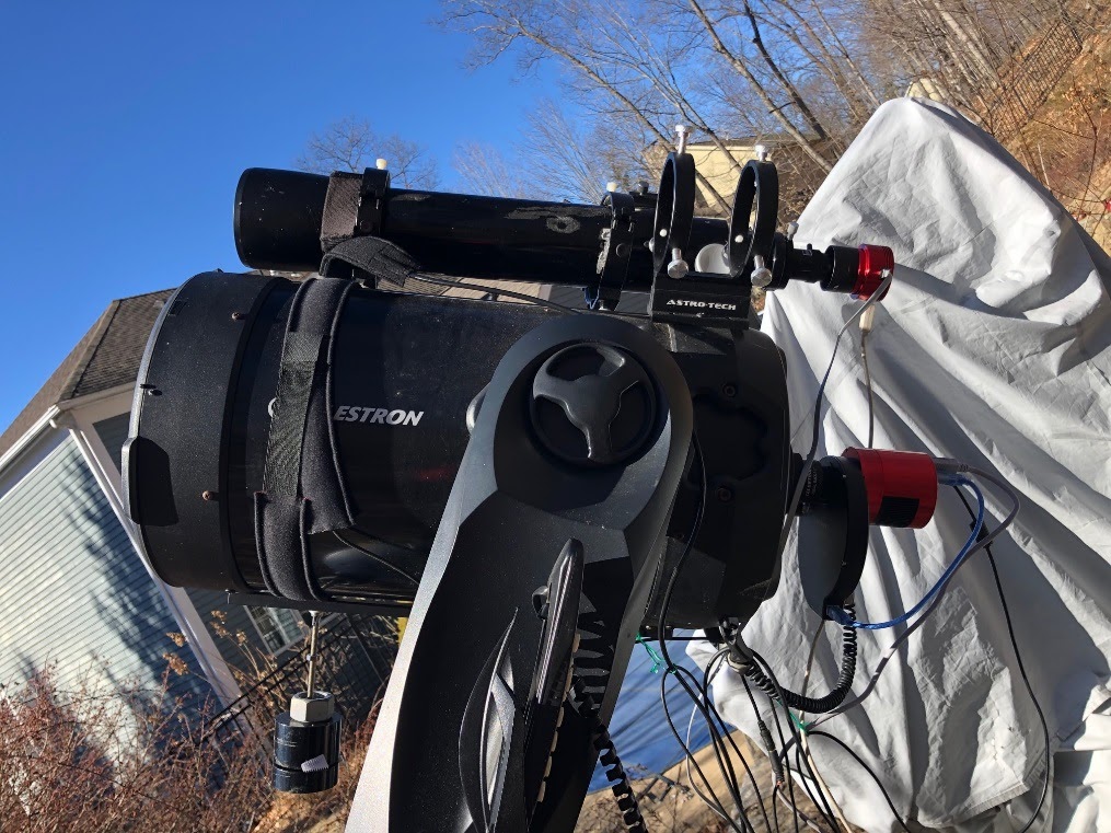
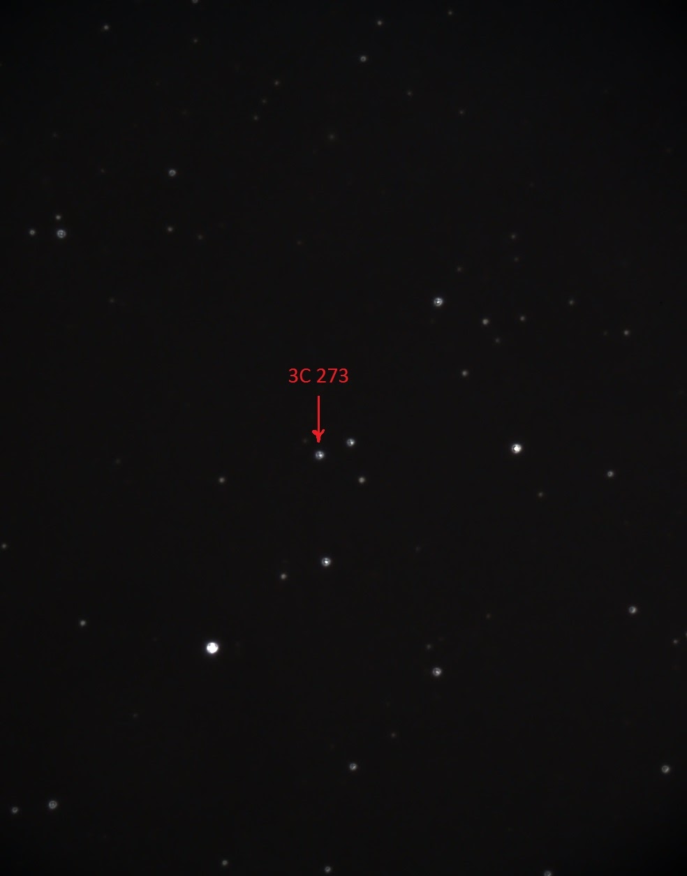
One of the first quasars ever detected was 3C 273 in 1963. This object is in the constellation Virgo and was originally labeled by the Tycho stellar catalog as TYC 0282-0202 when it was believed it was just an ordinary star. Even the most powerful telescopes on Earth just show this like a dim star because it is so far away. Astronomers use the magnitude scale to measure how bright stars are, and if we were in a very dark place on Earth, such as the North Pole, we could see up to magnitude 6, with the brightest stars in the sky at about magnitude 0 or 1, which we can see from New York City. 3C 273 is magnitude 12.9, which means you need a good telescope to see it. To image this object I used a Celestron CPC 11 telescope with a 0.63x reducer for an effective focal length of approximately 1700mm. The imaging camera was a ZWO 294mc Pro cooled to -10 and using about 300 gain. The spectrograph grating used was a Star Analyser 200; the average exposures were 1 minute, and I stacked about 40 frames. This camera and telescope combination can easily image down to 19 magnitude, so capturing the quasar normally is not a big deal given that it’s a rather bright 12.9 magnitude. Figure 3 below shows the scope and camera. I also have a stacked image and crop of the region around the quasar with 3C 273 highlighted in the center of the frame. Using a grating or similar spectrograph reduces the limiting magnitude by 4 to 5 magnitudes, so there probably is a limit to using this combination, down to maybe a 15 magnitude quasar.
Figure 3. CPC11 telescope and 3C 273 quasar image on right
So how exactly can we use physics and science to determine how far away 3C 273 is?
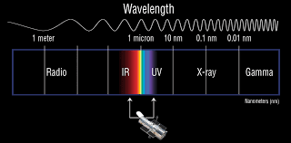
This is where chemistry and physics come together in using spectroscopy, or really, just looking at the spectrum of light from the quasar to determine its distance. All light can be broken down into its component colors based on the frequency of the light. The human eye can detect light from basically 400 to 700 nanometers. We call this the visible spectrum (Figure 4).
Figure 4. Visible spectrum
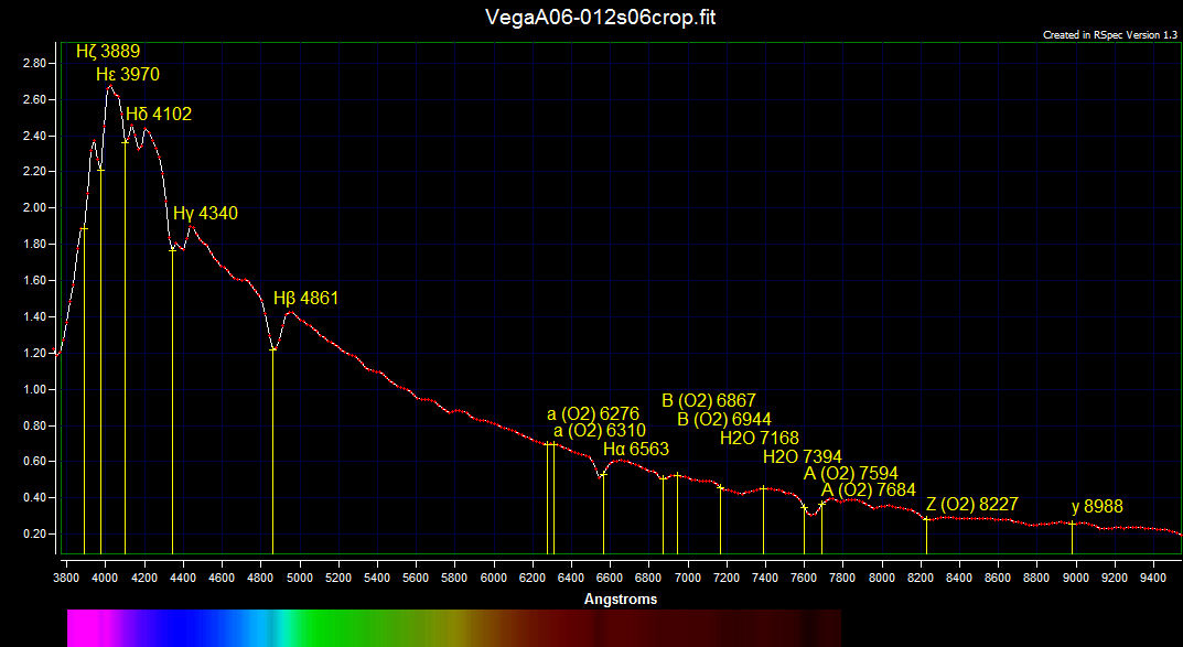
Now we can use the fact that certain wavelengths of elements can be detected in spectra as dark lines. These dark lines show absorption of certain elements and isotopes of elements like hydrogen or oxygen and many others. But what makes star spectra very usable is that every type of star has a unique type of spectrum based on its temperature. This means we can read the spectrum of a star and identify certain types of elements present in its emission of light. Below is the spectrum of a bright A0 type of star (Figure 5). We use a known star type such as this example of an A0-type star to calibrate our spectroscopic software, as different types of stars exhibit specific spectral features as the dark lines you can see below, each line identifying an element or isotope.
Figure 5: Spectrum of an A0 type of star like Alphecca or Vega
We can then use a special kind of filter with a tiny grating that splits the star light into a spectrum like that above. For my project I used the bright star Alphecca in the constellation Coronae Borealis. This star is not that far away, just 75 lightyears, and is very bright because it is a giant type of star over 2.6x larger than our sun. I took a photograph of this star using the special grating filter and obtained the spectrum you see below.
Figure 6. Alphecca spectrum
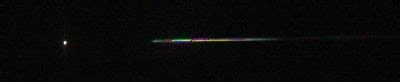
The spectrum is produced by imaging the starlight through a filter that has a very narrow grating built in which splits the starlight into its component colors as seen above. The grating I am using is from RSPEC and a “Star Analyser 200” (Figure 7).
Figure 7. Grating used to obtain the spectrum

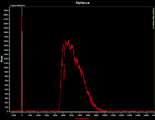
I then can use a different program to calibrate this spectrum and plot it using Angstroms as the x-unit value (Figure 8). Now, what is neat, the transformation of the color line to a graph will show the dark lines in the spectrum as dips in the curve. I have identified the dip below at 4,851 angstroms as Hydrogen-Beta. The hydrogen-beta emission line appears when a hydrogen atom falls from the 4th electron shell orbit to the 2nd. We know that the hydrogen-beta emission line occurs at 4,851 angstroms, so we can use this to calibrate our reference star (in this case, Alphecca with our target – 3C 273).
Figure 8: Alphecca calibration
While spectra can all be different, the part in the spectrum where these physical processes happen, such as a hydrogen electron falling from the 4th shell orbit the 2nd, is a constant in physics across the universe. So, if we are able to match the spectral line where the hydrogen-beta emission falls, we should be able to match any two stars and determine their relative distance from us as a function of this shift. We have learned about this shift in our physics class as the Doppler effect.
In astrophysics, the Doppler effect causes starlight to shift; that means that those telltale lines in the spectrum of stars will shift based on whether the star or object is moving toward you or moving away or is at rest (Figure 9).
Figure 9. Doppler effect in spectra

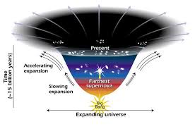
In Figure 9, the hydrogen-beta line is the third line from the left, highlighted by the end of the arrow. It can be seen how it moves to the right if it is redshifted, or moving away from you. This effect happens in the universe because it is thought that the universe is expanding. Think of the universe as the outside of a large balloon. When the Big Bang happened, the balloon started to inflate. If you are looking at an object across the universe you are also looking back in time when the balloon was not as inflated as it is now.
Figure 10. Universe expansion like a balloon
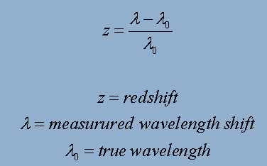
In the 1920s a young astronomer called Edwin Hubble discovered this idea. He wrote an equation that we use today to measure vast distances across the universe. All we need to do is measure the change in the redshift of the wavelength we are observing (Figure 12).
Figure 12. Change in wavelength equation
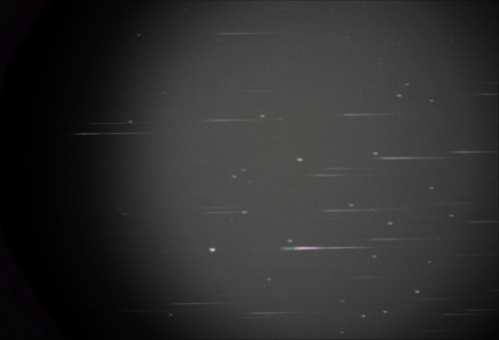
This is where we go back to our friend the quasar, 3C 273. Let’s take that image we took of the starlight, and run it through our special grating to split the starlight into a spectrum (Figure 13).
Figure 13. Telescope image of the 3C 273 and the stars around it by spectrum
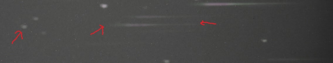
Of course, we want to isolate the quasar, 3C 273. This is what that looks like (Figure 14).
Figure 14. Quasar 3C 273 – spectrum detail
The last step is to plot this spectrum in our chart and in Angstroms and then to compare its spectrum and emission lines; in this case we are using hydrogen-beta to our reference star, Alphecca (Figure 15).
Figure 15. Quasar 3C 273 and Alphecca: comparison of hydrogen-beta lines
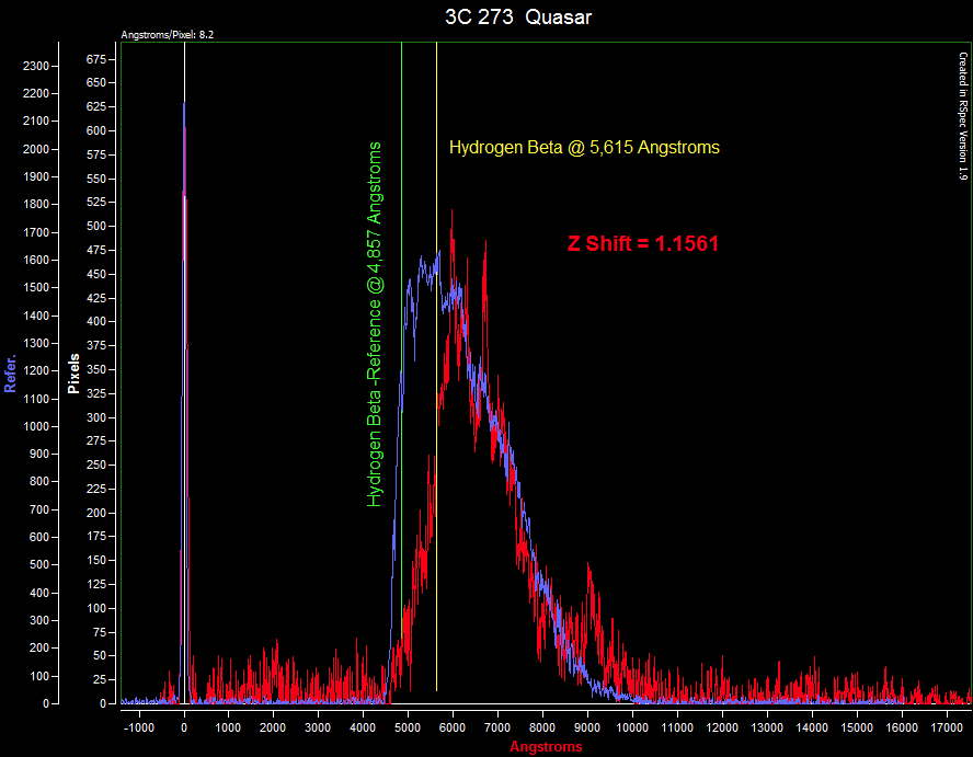
As we can see, the hydrogen-beta emission of 3C 273 occurs at 5,615 Angstroms, whereas the hydrogen-beta of the reference star is at 4,857 Angstroms. So, we can calculate the redshift or “Z” at 1.1561 or 0.1561.
The Hubble law states that the relationship of redshift to distance is: where d = distance, v = velocity, and H0 is the Hubble Constant of 72 km/s/megaparsec (mpc). A megaparsec is 3.26 million lightyears).
The velocity is 0.1561 times the speed of light. So, that is 0.1561 x 3 x 10^5 km/s or 46,830 km/s.
Now we can use the Hubble law, and plug in 46,830 km/s / 72 km/s/mpc. This equals: 650.42 megaparsecs x 3.26 million light years or 2.12 billion light years away!!
According to the most current sources, the actual measured redshift of 3C 273 is 0.158339, which means our modest amateur attempt came within 1.4% of the actual professional astronomer result, or in lightyears, we were about 30 lightyears off the mark…not bad!